


Transformers for Dummies: Multi-Headed Attention
Let's unpack the layer that made Transformers legendary in NLP

Consider the following sentence:
My mama always said life was like a box of chocolates, you never know what you’re gonna get
If I were to ask you who said this sentence, you’re most likely to not pay attention to every single word when deciphering the answer to this question, only to some key words in the sentence. The word “mama”, and the phrase “box of chocolates”, are enough to deduce that these words were spoken by our beloved Forrest Gump (unless of course, you haven’t seen the movie. In that case, I highly recommend watching this cinematic masterpiece).
Similarly, the attention mechanism helps a model focus on words that are most important in a sentence or words that give enough information to solve the task at hand.
Transformers go a step further and use “Self-Attention” mechanism.
Self-Attention
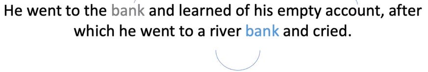
Let’s consider this sentence:

Notice how the word “bank” means two different things here. The first is a financial institution, and the second refers to a side of a river.
How does the model figure out which bank refers to what? The same way humans do - by paying attention to the context in which it appears. If you pay attention to the word “account”, you figure out that the first occurrence of the bank refers to a financial institute.
The word river can give a clue that the second occurrence of bank refers to land on a river’s side.
What is the difference between simple-attention and self-attention?
Say, our query was “Who is this Game of Thrones character?” and the sentence was “She faced her enemy and whispered - DRACARYS”.

Just by paying attention to the words, “She”, “enemy” and “DRACARYS”, anyone remotely aware of GOT can tell it was spoken by the mother of dragons, Daenerys Targaryen. This is exactly what simple attention does.
Simple attention pays attention to the words w.r.t some external query. The more important a word is in determining the answer to that query, the more attention is given to that word.
On the other hand, self-attention also takes the relationship of a word with other words in the same sentence into account.
![[video-to-gif output image]](https://substackcdn.com/image/fetch/$s_!XOER!,f_auto,q_auto:good,fl_progressive:steep/https%3A%2F%2Fsubstack-post-media.s3.amazonaws.com%2Fpublic%2Fimages%2F1b78e062-c987-434d-aa58-f79b8f38d56e_600x125.gif "[video-to-gif output image]")
Inside a Self-Attention Layer
Now that we have a bit of intuition about what self-attention means, let’s look into the actual blocks that make up a self-attention layer.
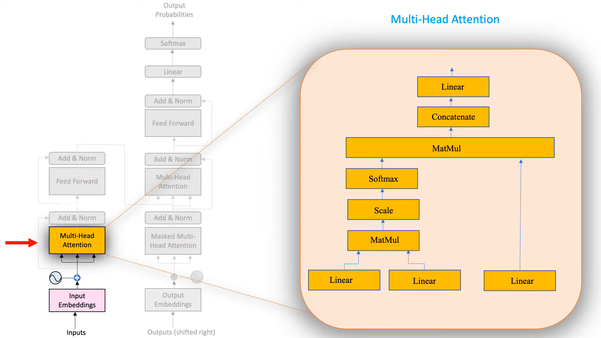
As you can see, there are quite a bit of blocks in there. We will go through them one by one.
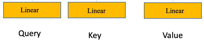
First up, we have three linear layers.
Why are we using linear layers?
In the case of Transformers, linear layers are used to shrink the size of the input which lowers computational cost. The bigger the input size i.e. the bigger the matrix, the more computation time and power it takes.
Each input (the input embeddings + positional embedding from the previous layer) is connected to the nodes via a weight. These weights are just what the model updates during training to get better and better at the downstream task. These weights are randomly initialized and fed to the model as a matrix.

Coming back to the Self-Attention layer’s blocks, we can see that there are three linear layers. They each have a different function and are called Query, Key, and Value respectively.
This can be motivated by the way retrieval systems work. Let’s take the example of searching for a video on YouTube. You type ‘k-means clustering’ in the search bar. Let us call this the Query.
For a moment assume that YouTube has a very simple algorithm. It goes through each video’s title and calculates its similarity with the Query. Then, it returns the video with the highest similarity to the Query. We can consider this video’s title to be the Key and its contents the “Value”.
![[video-to-gif output image]](https://substackcdn.com/image/fetch/$s_!p_Sa!,f_auto,q_auto:good,fl_progressive:steep/https%3A%2F%2Fsubstack-post-media.s3.amazonaws.com%2Fpublic%2Fimages%2F98d50217-8992-47aa-b7a9-1a3c74385e94_600x338.gif "[video-to-gif output image]")
Notice how similarity can serve as a proxy for attention.1
Coming back to Transformers, how do we calculate the similarity between a Query and a Key?
One great way is Cosine Similarity.
Cosine Similarity
It takes on values from +1 to -1 with +1 being most similar and -1 being most dissimilar.
When two vectors point in the same direction, the angle between them is zero. If you remember high school trigonometry, you know that cos(0) = 1. As the vectors move further apart from each other, the cosine similarity decreases. The highest dissimilarity occurs when the vectors point in the opposite direction.
![[video-to-gif output image]](https://substackcdn.com/image/fetch/$s_!kEn_!,f_auto,q_auto:good,fl_progressive:steep/https%3A%2F%2Fsubstack-post-media.s3.amazonaws.com%2Fpublic%2Fimages%2Fac92e17f-826a-4b8a-b265-cd5b9d85bb85_600x338.gif "[video-to-gif output image]")
Similarity between two matrices can be computed by:
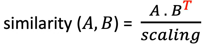
Let’s plug our Query and Key into our equation:

Before doing all these computations, we have to make three copies of the word embedding matrix and pass it through the Query, Key, and Value layers.
Now, you might be wondering that in our YouTube example, Query, Key, and Value had different contents. So why are we passing the same matrix to all three of them? This is where the “Self-Attention” mechanism comes in.
So we have 3 copies of our word embeddings. We pass each of them through a linear layer. We now call these the Query, Key, and Value matrices respectively. Next, we transpose our Key Matrix and multiply it with our Query Matrix (we need to transpose it so that we don’t run into matrix dimension incompatibility issues).
![[video-to-gif output image]](https://substackcdn.com/image/fetch/$s_!AHpn!,f_auto,q_auto:good,fl_progressive:steep/https%3A%2F%2Fsubstack-post-media.s3.amazonaws.com%2Fpublic%2Fimages%2Fdc6c5491-cad5-4c9b-9b18-f98e81ec28c7_600x338.gif "[video-to-gif output image]")
The output of this computation is an Attention Filter.
The contents of the Attention Filter are random at first. They are computed from word embeddings and word embeddings are random initially. It is after training that these numbers represent some meaningful value. These numbers are now called the “Attention Scores”. Take a look at the game row. It has the highest Attention Score with itself because a word is most similar to itself. The next highest score is given to the word “play”, which is the second most similar word to “game” (similar in the sense that they appear in the same context again and again).
![[video-to-gif output image]](https://substackcdn.com/image/fetch/$s_!MqTZ!,f_auto,q_auto:good,fl_progressive:steep/https%3A%2F%2Fsubstack-post-media.s3.amazonaws.com%2Fpublic%2Fimages%2Fab18aaed-7d85-48a5-aa09-1db8ed675533_600x338.gif "[video-to-gif output image]")
Next, the attention scores are scaled by sqrt(d_k) (each element is divided by sqrt(d_k)) where d_k is the dimension of the Key Matrix.
So basically, we have computed the Cosine Similarity of a sentence with itself.
We pass these Attention Scores through the softmax layer to squash the values between 0 and 1.
![[video-to-gif output image]](https://substackcdn.com/image/fetch/$s_!fPVk!,f_auto,q_auto:good,fl_progressive:steep/https%3A%2F%2Fsubstack-post-media.s3.amazonaws.com%2Fpublic%2Fimages%2F653924d0-4f32-4bcd-a8af-e41d1e16cff1_502x500.gif "[video-to-gif output image]")
Let’s do a quick recap:
We made 3 copies of the word embedding matrix and plugged them into three separate linear layers. Then we take the output of two of these linear layers and pass them through MATMUL, Scale, and Softmax layers which outputs the Attention Filter. The third copy of the word embedding is only passed through the linear layer.
Now, we have the following two matrices:
The Attention Filter
The Value Matrix
We’re now gonna go ahead and multiply these two. Although we are in the realm of NLP, the intuition behind this is best understood using computer vision.
Say you had to identify zebra crossing from these images to prove that you are not a robot:
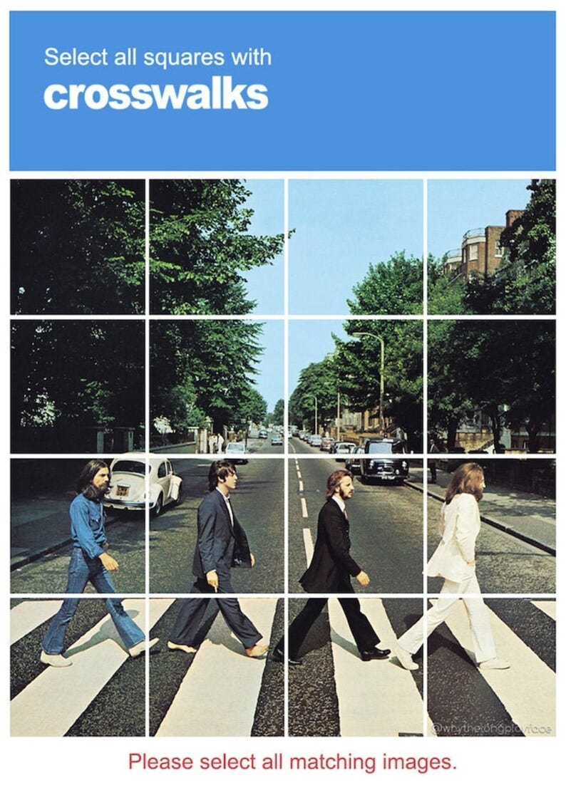
If you were to scan each image pixel by pixel, it would take you quite some time to get through this.
Instead, our brain, which is the most complex neural network out there, only pays attention to places where it can see some white stripes.

It won’t pay much heed to the four gentlemen or the blue skies because it knows they’re irrelevant to the task at hand.
If you look closely, this filtered image is a product of these two images:

The final filtered image only has the important and relevant stuff in it. Based on this information, you simply go ahead and select the bottom four tiles.
In a similar manner, we have our attention filter and our original value, we multiply them and get the filtered value. In this final filtered value, the most important features are assigned higher values.

The following formula sums up the computations in a single attention head:

Now, what we have talked about so far is one attention head. Transformers didn’t conquer the world of NLP using just one attention head, it uses a multi-headed attention layer.
Do we really need multi-headed attention or the authors of “Attention is All You Need” were just being fancy?
Well.
We’re trying to replicate a human brain here (more precisely, how a human brain processes language), nobody said it was going to be easy.
Transformers have multiple attention heads (in their attention layer) and each attention head learns a different set of linguistic phenomena. Each attention filter generates its own filtered value. Each zooming in on a different combination of linguistic features.
![[video-to-gif output image]](https://substackcdn.com/image/fetch/$s_!Qt58!,f_auto,q_auto:good,fl_progressive:steep/https%3A%2F%2Fsubstack-post-media.s3.amazonaws.com%2Fpublic%2Fimages%2Ff2438eff-6942-4666-818d-6e05d390a671_600x297.gif "[video-to-gif output image]")
The authors chose to use 8 attention heads (after a great deal of hyparameter tuning) but for our example, let’s stick to 3 heads.
Outputs of the different heads are simply concatenated together - horizontally. Since the output would grow larger and larger with each added attention head, we pass these concatenated heads through a linear layer to shrink the matrix to a size compatible with the next layers ahead. In our case, we’re going for size 7x5.

This is the final output of the Multi-Headed Attention Layer - the iconic layer that paved the way for Large Language Models.
https://www.youtube.com/@HeduAI